K-Nearest Neighbor Classification in Scikit Learn

K-Nearest Neighbor (k-NN) presents a a simple straightforward instance-based learning. Often, a simple strategy produces a good result as well as acting as baseline performance.

This article doesn’t deliver new knowledge but an interpretation and bridge to others’ work. The reader need to understand the very basic of Machine Learning. Especially, code is done with scikit-learn.

In particular, KNN can be used in classification. The training data is vector in a multidimensional space with a class label. k is an user-defined constant. A test sample is classified based on a distance metric with k nearest samples from the training data. That distance metric can be Euclidean distance for continuous variables. As of discrete data, Hamming distance is a good choice.

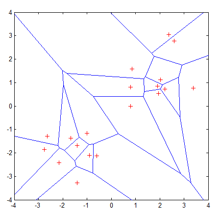
In Scholarpedia, it was visualized with Voronoi tessellation:

The k-nearest-neighbor classifier is commonly based on the Euclidean distance between a test sample and the specified training samples. Let \(\mathbf{x}_i\) be an input sample with \(p\) features \((\mathbf{x}_{i1},\mathbf{x}_{i2},\ldots,\mathbf{x}_{ip})\), \(n\) be the total number of input samples \((i=1,2,\ldots,n)\) and \(p\) the total number of features \((j=1,2,\ldots,p)\). The Euclidean distance between sample \(\mathbf{x}_i\) and \(\mathbf{x}_l (l=1,2,\ldots,n)\) is defined as

\(d(\mathbf{x}_i,\mathbf{x}_l)=\sqrt{(x_{i1}−x_{l1})^2+(x_{i2}−x_{l2})^2+\cdots+(x_{ip}−x_{lp})^2}\).

A graphic depiction of the nearest neighbor concept is illustrated in the Voronoi tessellation (Voronoi, 1907) shown in Figure. The tessellation shows 19 samples marked with a “+”, and the Voronoi cell, R , surrounding each sample. A Voronoi cell encapsulates all neighboring points that are nearest to each sample and is defined as

\(R_i=\{\mathbf{x}\in\mathbb{R}^p:d(\mathbf{x},\mathbf{x}_i) \leq d(x,x_m),\forall i \neq m\}\),

where \(R_i\) is the Voronoi cell for sample \(\mathbf{x}_i\), and \(x\) represents all possible points within Voronoi cell \(R_i\). Voronoi tessellations primarily reflect two characteristics of a coordinate system: i) all possible points within a sample’s Voronoi cell are the nearest neighboring points for that sample, and ii) for any sample, the nearest sample is determined by the closest Voronoi cell edge. Using the latter characteristic, the k-nearest-neighbor classification rule is to assign to a test sample the majority category label of its k nearest training samples. In practice, k is usually chosen to be odd, so as to avoid ties. The k = 1 rule is generally called the nearest-neighbor classification rule.

This is a great description of understanding. However I found out it’s misleading as visualization emphasizes too much on Voronoi instead of KNN itself.

How it works

It all comes out with the code. As in scikit-learn, the neighbors.KNeighborsClassifier(n_neighbors, algorithm='brute') implements the most simple way to use KNN. The class comprises of 4 mixins:

• SupervisedIntegerMixin: a helper checks parameters and invoke real function.
• ClassifierMixin: also a helper
• NeighborsBase: this mixin choose the optimal algorithm for efficient computing
• KNeighborsMixin: brute method is implemented here.

We only have to see how the brute with euclidean distance works to understand it.

X is the input here. self._fit_X is training data.

n_samples, _ = X.shape
sample_range = np.arange(n_samples)[:, None]
dist = pairwise_distances(X, self._fit_X, 'euclidean')
# here X is compared with all training samples.
# dist is like a matrix of distance from X to training samples.
# Example: `array([[1, 3, 2, 4]])`, 1 sample with 4 training data.

neigh_ind = np.argpartition(dist, n_neighbors - 1, axis=1)
# sort until `n_neighbors - 1`. When return, on the left side
# it should be smaller than this data point
neigh_ind = neigh_ind[:, :n_neighbors]
# argpartition doesn't guarantee sorted order, so we sort again
neigh_ind = neigh_ind[
    sample_range, np.argsort(dist[sample_range, neigh_ind])]

result = np.sqrt(dist[sample_range, neigh_ind]), neigh_ind

Staring from neigh_ind are some lines only used to sort result. At last, a distance result and the order of distance to training data is returned.

If you ever tried the sample code, you would notice the choice of k affects the result a lot upon iris dataset.

Plus, the weight metric and RadiusNeighborsClassifier is a further enhancement.

Conclusion

KNN is a really simple nearest neighbor classification or regression tool. It’s nothing fancy but with weight and algorithm you can tweak.